4. Graph¶

Graphs, or networks, show the structure of data through nodes and edges. Although they are very useful to show interconnections, matplotlib does not support them out of the box.

Multiplex’s graph visualization is built with the intent of making it easier to transform networks into stories. The Graph class supports both undirected and directed networks, styling and legends.

Note

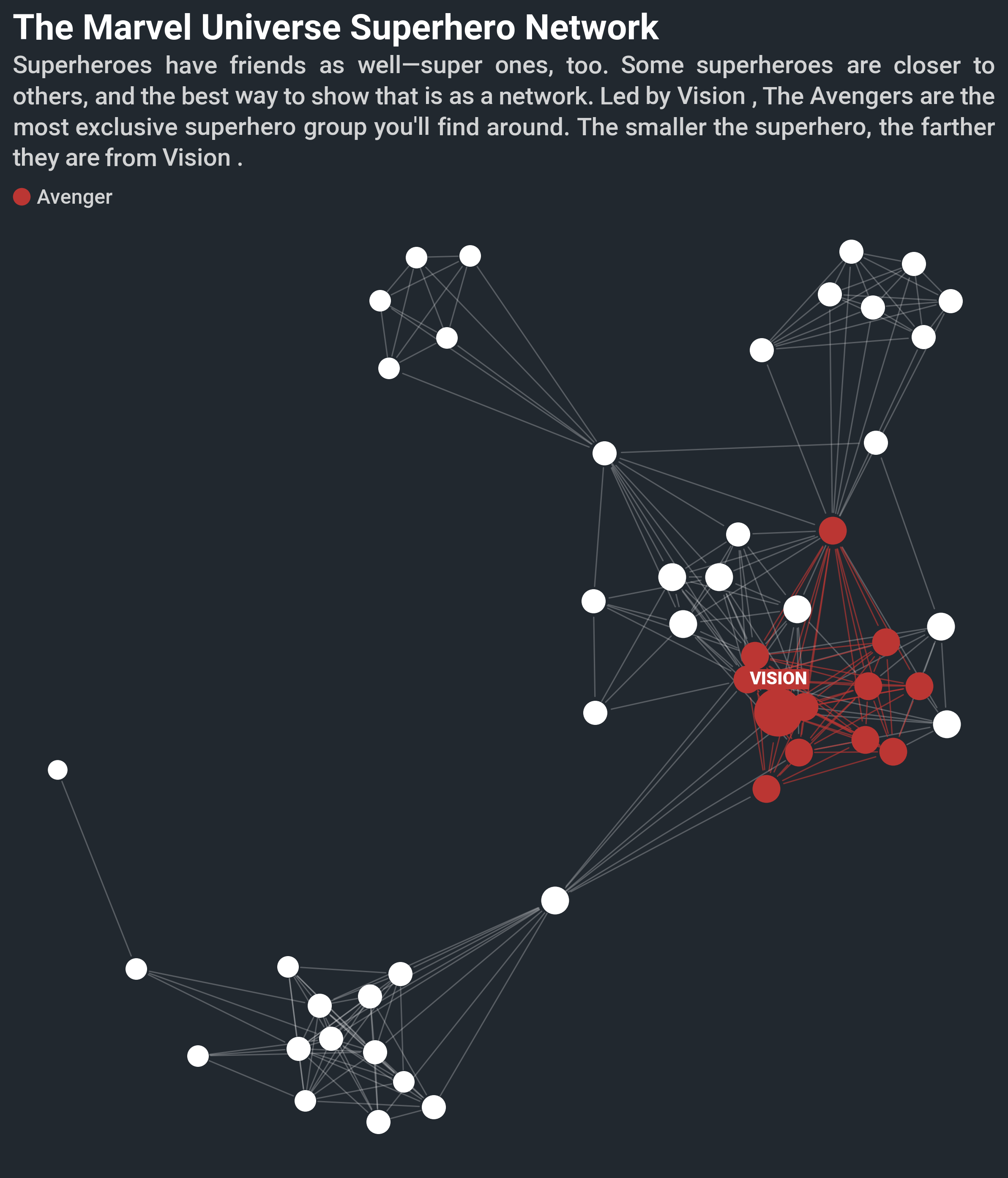
Multiplex’s Jupyter Notebook examples are a quick guide to get you up and running with creating network graph visualizations. Check out the network graph Jupyter Notebook tutorial to learn how to create the above visualization, or to start creating your own network graph visualizations.

Multiplex’s graph visualizations use the popular networkx library. If you already use networkx, you can visualize networks in a handful of lines:

import matplotlib.pyplot as plt
import networkx as nx
from multiplex import drawable
viz = drawable.Drawable(plt.figure(figsize=(10, 10)))
G = nx.path_graph(5)
viz.draw_graph(G, edge_style={ 'color': 'C1' },
               node_style={ 'color': 'C4', 'edgecolor': 'C1', 'linewidth': 2, 's': 250 })
viz.show()

Although Multiplex requires only the graph, you can style the nodes and the edges using the node_style and edge_style parameters.

Multiplex supports both undirected and directed edges. Moreover, the library also supports self-connections, or edges from a node to itself.

Apart from drawing nodes and edges, Multiplex is also capable of drawing names next to nodes and edges. These can be used, for instance, to write node names or describe the types of relations between nodes.

Finally, Multiplex’s graphs also support legend labels for both nodes and edges.

Warning

The graph visualization uses the networkx package to generate the layout of the graph. Therefore it is a prerequisite to have it installed before creating these visualizations.

class graph.graph.Graph(*args, **kwargs)¶

The Graph class is a general network graph that plots nodes and creates edges between them. Like all visualizations, it stores a Drawable instance and revolves around the draw() function.

The Graph class builds on the LabelledVisualization. The reason why the Graph builds on that, and not the simpler Visualization, is that it uses the LabelledVisualization’s labels for node names. In this way, the Graph automatically ensures that the node names do not overlap.

__init__(*args, **kwargs)¶: Initialize the graph.

draw(G, positions=None, node_style=None, name_style=None, edge_style=None, label_style=None, *args, **kwargs)¶

Draw the given networkx graph on the Drawable.

The method expects only a graph. Differently from other visualizations, the styling options are passed on as dict arguments.

By default, this method generates the node positions using the networkx.spring_layout function. The args and kwargs are passed on to this function to control how the graph looks. However, you can provide your own node positions in the positions argument.

To draw the graph, the Graph draws three types of components:

Nodes using matplotlib’s scatter function,

Undirected edges using matplotlib’s plot function and directed edges using matplotlib’s annotate function, and

Node and edge names using Annotation.

The Graph automatically draws names next to nodes and edges whenever it finds a name attribute. You can set the name directly on the node or edge in the graph:

G.nodes['u']['name'] = 'node'
G.edges[('u', 'v')]['name'] = 'edge'

Similarly, the Graph adds a legend for nodes and edges whenever it finds a label attribute. You can set the label directly on the node or edge in the graph:

G.nodes['u']['label'] = 'node'
G.edges[('u', 'v')]['label'] = 'edge'

Parameters:

G (networkx.classes.graph.Graph) – The networkx graph to draw. The function automatically detects whether the graph is undirected or directed and draws the edges accordingly.
positions (dict) –
The node’s initial positions. If you provide no positions, the function uses the networkx.spring_layout function to find the best position for nodes. If you provide a position for a subset of the nodes, the rest of the positions are generated automatically.

You can provide the positions with node names as keys and their positions as values. Positions must be tuples: the x and y coordinates.
node_style (dict) –

The general style for nodes.

The node_style accepts any styling option supported by matplotlib’s scatter function.

You can override the general style of the nodes by giving them a style attribute:
```
G.nodes['u']['style'] = { 'color': '#BB3633' }
```
Note

You can set the size of nodes by setting the s key in the node_style. By default, the size is 100.
name_style (dict) –

The general style for names.

The name_style accepts any styling option supported by the Annotation’s draw() function.

You can override the general style of the names by giving nodes and edges a name_style attribute:
```
G.nodes['u']['name_style'] = { 'fontweight': 'bold' }
G.edges[('u', 'v')]['name_style'] = { 'fontweight': 'bold' }
```
edge_style (dict) –

The general style for edges.

The edge_style accepts any styling option supported by matplotlib’s plot and annotate functions.

You can override the general style of the edges by giving them a style attribute:
```
G.edges[('u', 'v')]['style'] = { 'color': '#BB3633' }
```
label_style (dict or None) – The general style for labels. The label_style accepts any styling option supported by the Annotation’s draw() function.

Returns:

A tuple containing the drawn components:

A list of drawn nodes as matplotlib.collections.PathCollection instances,
A list of rendered node names as Annotation instances,
A list of edges as matplotlib.lines.Line2D instances if the graph is undirected or as matplotlib.text.Annotation if the graph is directed, and
A list of rendered edge names as Annotation instances.

Return type:

tuple